BIND 9.20 Resolver performance compared to 9.18

In this post, we will show that BIND 9.20 compares favorably with 9.18, providing faster responses to clients, both with a cold cache and after the cache is filled. In low-traffic scenarios, BIND 9.20 can consume more memory than 9.18, but as traffic increases, BIND 9.20 uses less memory than BIND 9.18.

We run performance tests continually as part of our development process, but the detailed results are more relevant to the development team than to users. Periodically we publish performance benchmarks so that users considering an upgrade can assess the likely performance change in their own deployment.

This article focuses on benchmarking resolver performance, using a methodology that aims to provide near-real-world performance results for resolvers. Our methodology has not changed significantly since our 2021 blog post, but for ease of reading we have repeated the description of the test methodology. If you are already familiar with our test methodology, scroll down until you see the charts for the results.

About Resolver Testing

Cache State and Timing Matter

Resolvers don’t know any DNS answers by themselves; they have to contact authoritative servers to obtain individual bits of information and then use them to assemble the final answer. Resolvers are built around the concept of DNS caching. The cache stores DNS records previously retrieved from authoritative servers. Individual records are stored in a cache up to the time limit specified by the authoritative server (Time To Live, or TTL). Caching greatly improves scalability.

Any DNS query which can be fully answered from cache (a so-called “cache hit”) is answered blazingly fast from the DNS resolver’s memory. On the other hand, any DNS query which requires a round-trip to authoritative servers (a “cache miss”) is bound to be orders of magnitude slower. Moreover, cache miss queries consume more resources because the resolver has to keep the intermediate query state in its memory until all information arrives.

This very principle of the DNS resolver has significant implications for benchmarking: in theoretical terms, each DNS query potentially changes the state of the DNS resolver cache, depending on its timing. In other words, queries are not independent of each other. Any change to how (and when) we query the resolver can impact measurement results.

In more practical terms, this implies a list of variables that we have to replicate:

• A stream of test queries resulting in a realistic cache hit/miss rate. For this purpose, we have to replicate the exact queries and also their timing.
• Answers returned by authoritative servers, including TTL values.
• Network conditions between the resolver and authoritative servers (latency, packet loss, etc.).
• Cache size and other parameters affecting cache hit/miss ratio.

The traditional approach implemented, e.g., in ISC’s Perflab or using the venerable resperf tool, cannot provide realistic results because it ignores most of these variables.

The second implication is that even the traditional QPS metric (queries answered per second) alone is too limited when evaluating resolver performance: it does not express the type of queries, answer sizes and TTLs, query timing, etc.

You Can’t Simulate the Internet

The long list of variables above makes it clear that preparing an isolated laboratory with a realistic test setup is very hard. In fact, ISC and other DNS vendors have learned that it’s impossible; realistic resolver benchmarking must be done on the live Internet.

Developers from CZ.NIC Labs wrote a test tool called DNS Shotgun for this purpose. It replays DNS queries from traffic captures and simulates individual DNS clients, including their original query timing. The resolver under test then processes queries as usual, i.e., contacts authoritative servers on the Internet and sends answers back to the simulated clients. DNS Shotgun then receives and analyzes the answers.

Obviously, benchmarking on a live network cannot provide us with perfectly stable results. To counter that, we repeat each test several times and always take fresh measurements instead of using historical data. This process ensures that changes on the Internet and our test system do not skew our comparison.

For each test run, we start with a new resolver instance with an empty cache. This way, we simulate the worst case of regular operation: it is as if the resolver was restarted and now has to rebuild its cache from ground zero.

Let’s have a look at the variables we measure and how to interpret them.

Interpreting Resolver Behavior

The QPS metric alone is not particularly meaningful in the context of regular DNS resolver operation. Instead, we measure indications that resolver clients are getting timely answers, and resource consumption on the server.

a) CPU Utilization

We monitor time BIND processes spent using the CPU as reported by the Linux kernel Control Group version 2 metric usage_usec, and then normalize the value in a way which gives 100 % utilization = 1 fully utilized CPU. Our test machine has 16 cores, so its theoretical maximum is 1600 %. CPU usage is a cumulative metric and we plot a new data point every 0.1 seconds.

b) Memory Usage

We use the Linux kernel Control Group version 2 metric memory.current to monitor BIND 9’s memory consumption. It is documented as “the total amount of memory currently being used” and thus includes memory used by the kernel itself to support the named process, as well as network buffers used by BIND. Resolution of the resource monitoring data is 0.1 seconds, but the memory consumption metric is a point-in-time value, so hypothetical memory usage spikes shorter than 0.1 seconds would not show on our plots.

c) Response Latency - How quickly does the resolver respond?

Finally, we arrive at the most useful but also the most convoluted metric: response latency, which directly affects user experience. Unfortunately, DNS latency is wildly non-linear: most answers will arrive within a split-millisecond range for all cache hits. Latency increases to a range of tens to hundreds of milliseconds for normal cache misses and reaches its maximum, in the range of seconds, for cache misses which force communication with very slow or broken authoritative servers.

This inherent nonlinearity also implies that the simplest tools from descriptive statistics do not provide informative results.

To deal with this complexity, the fine people from PowerDNS developed a logarithmic percentile histogram which visualizes response latency. It allows us to see things such as:

• 95 % of queries were answered within 1 ms (cache hits)
• 99 % of queries were answered within 100 ms (typical cache misses)
• 99.5 % of queries were answered within 1000 ms (problematic cache misses)

and so on.

Even more importantly, a logarithmic percentile histogram allows us to compare the latency of various resolver setups visually.

Test Methodology

Data Set and Load Factor

For realistic results, we need a realistic query data set. This article presents results measured using traffic captures (of course anonymized!) provided by one European telecommunications operator. We would really love any samples other operators could provide, as diversity in our sample data would make our testing more representative.

These traffic captures contain one hour of traffic directed to 10 independent DNS resolvers, all of them with roughly the same influx of queries. In practice, we have 10 PCAP files: the first with queries originally directed for resolver #1, the second with queries directed to resolver #2, etc.

These traffic captures define the basic “load unit” we use throughout this article: traffic directed to one server = load factor 1x. To simulate higher load on the resolver, we simultaneously replay traffic originally directed to N resolvers to our single resolver instance under test, thus increasing load N times. E.g., if we are testing a resolver under load factor 3x, we simultaneously replay traffic originally directed to resolvers #1, #2, and #3.

This definition of load factor allows us to avoid theoretical metrics like QPS and simulate realistic scenarios. For example, it allows us to test this scenario: “What performance will we get if nine out of 10 resolvers have an outage and the last resolver has to handle all the traffic?”¹

Test Design

Here is the basic testbed setup we used to compare the most recent release of BIND 9.20 to the most recent BIND 9.18 version. We intentionally are not providing the exact hardware specifications to prevent readers from an undue generalization of results.

• We use two servers: one to simulate (many) DNS clients using DNS Shotgun, and the other to run the DNS resolver under test.
• Each machine has 16 logical CPUs (eight physical cores with hyperthreading enabled) and 42 GB of operating memory.
• DNS Shotgun is configured to replay the original query stream (including timing) from one or more (original) telco resolvers to one machine running a resolver under test, with 2000 ms timeout on the client-side.²
• BIND is configured with max-cache-size set to 30 gigabytes. Practically, all other values are left at default settings: the resolver is doing full recursion and DNSSEC validation. Also, the resolver has both IPv4 and IPv6 connectivity.
• The resolver and client machine always start from a completely clean state; most importantly, the resolver always starts with an empty cache. This approach allows us to measure the worst-case scenario, “how quickly will the resolver recover after a restart?” In practice, we inspect resolver behavior in the first 600 seconds, and expect service recovery within the first 60 seconds. Of course, 600 seconds is a short test compared to regular resolver uptime. We are focusing on the worst-case scenario, which is an empty cache. Depending on client behavior, the resolver can handle even more load after it has had more time to fill its cache. By starting in a clean state, we ensure that the performance levels described in this article can be safely reached without worrying about system restarts, complicated load balancing, etc.

There is one point I cannot stress enough:

Individual test results like response rate, answer latency, maximum QPS, etc., are generally valid only for the specific combination of all test parameters, the input data set, and the specific point in time.
In other words, results obtained using this method are helpful ONLY for relative comparison between versions, configurations, etc., measured on the exact same setup with precisely the same data and time.

For example, a test indicates that a residential ISP setup with a resolver on a 16-core machine can handle 160k QPS. It’s not correct to generalize this to another scenario and say, “a resolver on the same machine will handle a population of IoT devices with 160k QPS on average” because it very much depends on the behavior of the clients. If all of our hypothetical IoT devices query every second for api.vendor.example.com AAAA, the resolver will surely handle the traffic because all queries cause a cache hit. On the other hand, if each device queries for a unique name every second, all queries will cause a cache miss and the throughput will be much lower. Even historical results for the very same setup are not necessarily comparable because “something” might have changed on the Internet.

Please allow me to repeat myself:

This test was designed to compare BIND 9.18 to BIND 9.20, handling a specific set of client queries at a specific point in time. Depending on the test parameters and your client population, your results could be completely different, which is why we recommend you test yourself if you can.

Results

We have eight sets of charts, all using the one query data set. We ran the test in a long (600 second) duration, with 1x, 5x and 20x load factors. Then we ran the same test in short (120 second) duration, using load factors 1x, 5x, 10x, 15x and 20x. The longer duration tests are more useful to checking on memory consumption as the cache has time to fully populate, and CPU utilization over time, but the shorter tests are fine for measuring response latency.

Charts shown in this section show aggregate results from three repetitions of the test on each version. The full line shows the average of the three tests, while the colored background shows the range between minimum and maximum for each version. That is, the wider the color background is, the more unpredictable the characteristic is, and vice versa.

CPU utilization

Let’s have a look at CPU load during the longer ten-minute test. We have charts for the base, 5x, and 10x load factors. Remember, our test machine has 16 cores, so its theoretical maximum is 1600 %.

Base load factor

This chart shows CPU load, test times 0 - 600 seconds, with the base load factor. Utilization is around 60% and slightly lower for BIND 9.20 vs 9.18.

5x load factor

This chart shows the same test, with 5x the base load. CPU utilization is around 200%, nearly the same for both versions.

20x load factor - note the colors are reversed, 9.20 is orange here**

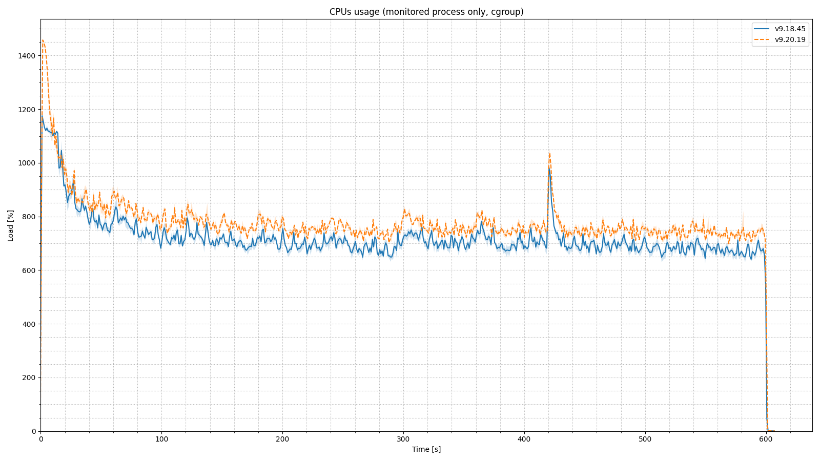
In the 20x load factor scenario, on start-up, BIND 9.20 makes better usage of the CPU, spiking much higher than 9.18. CPU utilization stabilizes at 650 - 800% for the duration of the test, slightly higher for the more recent BIND version. (We ran this test after the first batch of tests, which is why the chart is formatted differently.)

Memory usage

Similarly to CPU usage, we use the longer 10-minute test run to look at memory usage.

Base load factor

In our base load factor scenario, BIND 9.20 uses more memory than 9.18. Note that memory usage is expected to grow over time as the cache fills up with records.

5x load factor

In the 5x load factor scenario, BIND 9.20 initially uses less memory than 9.18, while the cache is cold. By the end of the 10-minute test, with the cache fully warm, 9.20 is using more memory, roughly 800 MB vs approximately 750 MB for 9.18. The memory differential with BIND 9.20 is much lower on a busy resolver than on the less-busy base load factor.

20x load factor - 9.20 is orange here

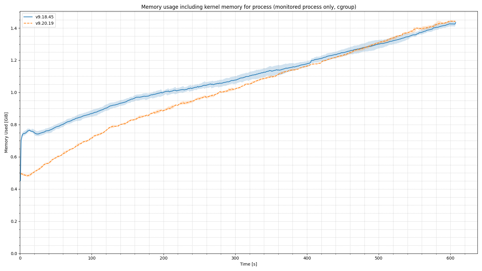
In the 20x load factor scenario, BIND 9.20 again uses quite a bit less memory than 9.18 at startup, when the cache is empty. By the end of the test, both BIND versions are using the same amount of memory (within our test variance). Therefore, a heavily loaded resolver should expect to see no difference in memory usage when moving from 9.18 to 9.20, while running in a steady state.

Response latency - How quickly does the resolver respond?

These are the most important charts, since the goal of the service is to answer the most clients as quickly as possible. On these charts, the lines that are closer to the left side of the chart are showing lower latency for more users, which is a better result. In the lower right corner you see the large percentage of queries that are answered in two milliseconds or less; these queries are presumably answered from the local cache. Our test is not designed to differentiate at the level of a millisecond or two, so the shape of the curve below two milliseconds is immaterial. As the line rises to the left, you see the percentage of queries that have to wait for resolution via the Internet. Flat lines on the top at the 2000 ms mark show client timeouts.

Cold cache

These charts show how BIND responds during the first 60 seconds after startup. The performance of BIND 9.20 is very similar to 9.18 in the base load factor scenario; only about 8% of queries remain to be answered after the first two milliseconds. This means this resolver is attaining a cache hit ratio of approximately 92 % within the first minute of operation.

At five times the base load factor, we see the best cache hit rate in our first minute of tests. Cache hit rate is dependent on the actual queries made, but since all of these tests use the same query set, you can see the impact of different query rates. Cache hit rates will increase across the board during the second minute, shown in the section below.

As we increase the load factor, the BIND 9.20 line moves further to the left of the BIND 9.18 line. When we test with 10x the base load factor, you can see that BIND 9.20 is answering about 3% more queries from cache than BIND 9.18, which means a smaller percentage of queries are resolved through queries from BIND to the Internet. Fewer than half as many queries time out in the upper left quadrant with BIND 9.20, versus 9.18.

By the time we increase the load to 20x our base, the BIND 9.20 server answers about 10% more queries within the first two milliseconds than 9.18. The overall cache hit rate is significantly worse with this heavy load. In the top left quadrant of the chart, you see that a quarter or fewer of the queries to 9.20 time out, compared with 9.18. This chart shows that BIND 9.20 handles the initial startup of a heavily loaded resolver much better than 9.18.

Warm cache

After the first minute, the cache is already populated with records and becomes “hot.” The following charts show response latency for the second minute of this two-minute test.

In the base load factor test, you get about a 1% improvement in answers from cache with BIND 9.20, but overall, response rates are very similar. The blue lines representing 9.20 are fairly consistently to the left of the orange lines, meaning the more recent version has lower latency.

As we increase the load to 5x, we see a further increase in the cache hit rate to about 97%. This demonstrates the benefit of running an active, busy resolver in reducing response time for users.

Cache hit rate peaks at 98% in the 10x base load scenario.

As the load increases, the number of queries that time out in BIND 9.20 eventually drops (seen in the upper left corner of the chart). These are small differences in the end of the long tail of responses. As expected, this second measurement at our highest traffic rate has a much higher cache hit rate, about 97%, than the measurement during the first minute of the test, which was 70-80%.

Our conclusion is that BIND 9.20, which included significant refactoring, including adoption of qp-trie in place of the red-black tree database, did not incur any resolver performance penalty, and actually provides lower-latency responses to clients than 9.18 did, particularly during the cold cache phase of operation.

References

• Release notes for BIND 9.20.0.
• BIND Administrative Reference Manual for 9.20.0.
• We have updated the BIND Significant Features Matrix.
• ISC’s Software Support Policy and Version Numbering explains the release cycle.